Model architectures: how we reached fine-grained MoEs and today's hybrids

Research and technical explanation. October 2026. A history of the decisions that changed computation, memory, and the circulation of information in language models.

A model with hundreds of billions of parameters may use only part of them to process a token. Another may traverse a long text without storing a key and value for every position in every layer. A third may combine these two choices.

Looking only at the parameter count hides this difference. Architecture determines where computation happens, what remains stored, and how information can influence the next response.

The history is also less linear than it looks. MoE did not appear after the Transformer; recurrent mechanisms did not disappear when attention gained scale. The lines developed in parallel and later began to be combined. To understand current architectures, we need to follow the problems each one tried to solve.

The years below follow the first version of the cited preprint or the indicated publication when there is no preprint. Model release dates are identified separately; do not confuse a paper's year with the year it was presented at a conference.

Before the timeline: three different accounts

When reading a model card, separate three resources:

• Weights: the learned parameters that need to be stored and accessed.

• Computation per token: the work performed to transform a representation and produce the output.

• Context state: what is retained from the sequence to continue processing or generating.

Reducing one of these accounts does not automatically reduce the others. MoE mainly acts on the selection of parameters in transformation networks. Sparse attention selects context positions. Recurrent mechanisms update a state. These choices can coexist.

There are also two different phases in autoregressive generation: prefill, when the model processes the input, and decode, when it continues the sequence. An efficient solution in the first phase may not behave the same way in the second.

1990–2014: recurrent memory and experts were already distinct lines

Recurrent networks process a sequence by updating an internal state. Elman's 1990 work is a milestone for this approach: the representation at one step participates in the next step's processing. This allows information to be carried through time, but creates sequential dependencies and difficulties in learning very distant relationships. It is not the absolute origin of every recurrent network. Elman, 1990 [1].

In 1997, LSTM introduced an organization of memory and gates to improve learning of long dependencies. The network learns to control the flow of information instead of simply replacing the whole state at each input. Memory remains finite; better control does not equal preserving every detail of a sequence without loss. LSTM [2].

Meanwhile, another question was already being investigated: do all examples need to use the same combination of networks? Jacobs and colleagues' 1991 work presented mixtures of local experts, with a mechanism for selection and combination. In 1994, Jordan and Jacobs published the hierarchical tree formulation. These precedents should not be described as if they were already the top-k MoE of today's large Transformers. MoE, 1991 [3], hierarchical mixtures, 1994 [4].

The questions were complementary: how to carry information through a sequence and how to divide work among parts of a network.

2014: attention eases the bottleneck of compressing everything into one vector

In the seq2seq model by Sutskever and colleagues, one LSTM encodes the input and another generates the output from that representation. The approach made it possible to learn transformations between sequences of different lengths. But concentrating the input information in a fixed-size representation imposed a bottleneck. Seq2seq [5].

In the same year, Bahdanau and colleagues introduced an alignment and attention mechanism that allows the decoder to consult representations at different input positions during generation. Instead of relying only on a single summary, the output can seek information at different points in the sequence. Attention for neural translation [6].

The two preprints are from September 2014. The order of exposition here explains the problem and the solution; it does not claim that the attention work was published after that seq2seq work.

2017–2019: the Transformer reorganizes processing

The 2017 Transformer made attention the central mechanism for communication among positions, without recurrence or convolution in the presented architecture. This favors parallel processing of positions during training, subject to masks. Attention Is All You Need [7].

A block combines attention, a feed-forward network — FFN, applied to the representations at each position —, residual connections, and normalization. Attention mixes information across positions; the FFN transforms each representation using that block's weights.

The original Transformer is encoder-decoder. The configurations that became known later explore different uses:

• Encoder, such as BERT: uses context from both sides to build representations, with the masking training described in the paper. BERT, 2018 [8].

• Decoder-only, such as the initial GPT: uses causal attention to predict the continuation without accessing future tokens. GPT, 2018 [9].

• Encoder-decoder, such as T5: organizes tasks as text-to-text transformation, with one side encoding and the other generating. T5, 2019 [10].

“Transformer” does not automatically mean causal attention. The mask and model organization determine what each position can consult.

What it means to be dense

In a conventional dense Transformer, tokens pass through the block's same dense transformations, without a router choosing subsets of expert FFNs. This is more precise than saying that literally every parameter participates in every token: embeddings involve lookups into rows of a table, for example.

There are also two different meanings of “dense”: a model may have dense FFNs and sparse attention, or MoE FFNs and full attention. The term needs to be accompanied by the component to which it refers.

Improvements such as RMSNorm, SwiGLU, and RoPE also changed the blocks. The 2023 LLaMA brings these choices together in a decoder Transformer. They affect training and processing, but do not, by themselves, turn a dense FFN into MoE. LLaMA [11].

2017–2023: sparse MoE gains scale

In January 2017, before the Transformer preprint, Shazeer and colleagues presented an MoE layer with sparse combinations of experts and thousands of possible subnetworks. The study includes a model of up to 137 billion parameters among LSTM layers. The story does not begin with only two or four experts. Sparsely-Gated MoE [12].

In MoE Transformers, it is common to replace certain FFNs with sets of expert FFNs. A router computes scores from the token representation, chooses some networks, and combines their outputs. Attention, normalization, and other parts of the block continue to participate in processing.

GShard, in 2020, explored the distributed scale of this combination. Switch Transformers, in 2021, studied a simplified route: select one expert per token, along with decisions needed for stable training. These are architecture and systems choices, not merely an increase in the number written on a specification sheet. GShard [13], Switch Transformers [14].

Mixtral 8×7B, announced in December 2023 and described in a January 2024 paper, made another design highly visible: eight experts per MoE layer, with two selected per token. The paper reports 46.7 billion total parameters and 12.9 billion active per token. “8×7B” does not mean eight independent complete 7B models running at the same time. Announcement [15], Mixtral paper [16].

An expert is a learned subnetwork, not necessarily a stable human department. Routing may reflect linguistic, syntactic, or task patterns without producing a readable division such as “this is legal, that is programming.”

2019–2023: attention, long context, and memory follow another path

Even with few active FFNs, the model must handle context. In full attention, the number of relations among positions grows quadratically with sequence length during joint processing, keeping the other dimensions fixed.

During decode with a KV cache, all old pairs are not recalculated for every token: the new token consults previous keys and values. The query grows with the history; the cache also occupies more memory as the sequence grows. This is a different cost from storing the weights. MQA and decoding cost [17].

Sharing keys and values: MQA and GQA

Multi-Query Attention, from 2019, shares keys and values among query heads. Grouped-Query Attention, from 2023, uses groups: several query heads share each KV set, offering an intermediate point between one KV head and one per query head. MQA [17], GQA [18].

This reduces the volume of KV to store and move. It does not mean that the model stopped consulting the positions allowed by its attention.

Choosing positions: Longformer and BigBird

In 2020, Longformer combined local windows with task-defined global attention. BigBird combined local, global, and random patterns. These are ways of building connections among positions without computing every pair. Longformer [19], BigBird [20].

A window allows examining the neighborhood; global or distant connections help information travel beyond it. The design needs to preserve the paths the task requires. “Not computing a connection” does not show that it would be irrelevant for every input.

Running the same attention better: FlashAttention

FlashAttention, from 2022, is another category of contribution: it reorganizes computation to reduce transfers among GPU memory levels without materializing the full attention matrix of the naive implementation. Its exact-attention algorithm does not automatically turn quadratic arithmetic into linear arithmetic. FlashAttention [21].

Changing the connections and improving the kernel that computes those connections are different decisions. An architecture delivers its practical gains only when the implementation and hardware can use them.

2020–2025: recurrence, convolutions, and structured memory return to the center

The 2020 paper Transformers are RNNs showed a formulation of linear attention with a recurrent interpretation. Reorganizing the operation allows updating a state instead of explicitly storing all relations. This involves attention different from conventional softmax, not a simple exact acceleration of the same formula. Linear Attention [22].

S4 and Mamba: state space with content selection

S4, in 2021, explored structured state-space models for long sequences. The idea is to represent a state's dynamics and its transformation into an output with a parameterization that permits efficient processing. S4 [23].

Mamba, presented in December 2023, added input-dependent selectivity: mechanisms that control how information enters, remains, and is read can change with the content. This selectivity requires a suitable processing algorithm; it is not merely reusing the convolution of a fixed linear system. Mamba [24].

Mamba-2, in 2024, developed the duality between state-space models and forms of structured attention through the SSD framework. The mathematical relation enables new algorithms; it does not show that every SSM and every Transformer are equivalent substitutes for every task. Mamba-2 and SSD [25].

In recurrent execution with fixed dimensions, the state of these layers does not grow with every token in the history. The price is representing the past in finite capacity instead of keeping a separate KV record for every position. Recovering an old detail exactly remains something to evaluate.

RetNet, RWKV, and DeltaNet: other ways to update memory

RetNet, in 2023, introduced a retention mechanism with parallel, recurrent, and chunkwise forms. RWKV explored a design that can be trained in parallel but infers recurrently. These are lines related to the search for sequence efficiency, not simply new names for Mamba. RetNet [26], RWKV [27].

Gated linear attention, such as GLA, allows modulating updates to a matrix state. DeltaNet, in 2024, explores a corrective memory-update rule; Gated DeltaNet, presented at ICLR 2025, combines corrective writing with adaptive forgetting. This offers different ways to control what is retained and replaced. GLA [28], DeltaNet [29], Gated DeltaNet [30].

Recurrent inference forms and parallel training algorithms are two faces of this engineering. A state of fixed size relative to history does not mean zero cost, nor training entirely with constant memory: dimensions, activations, blocks, and implementation strategy still matter.

Convolutions also continued to evolve

Hyena, from 2023, combines parameterized long convolutions and gates to mix information without conventional full attention. It is another line of sequence operators. Hyena [31].

The 2025 LFM2 report shows a different combination: many short gated-convolution layers and some GQA layers, aimed at device-execution constraints. Local convolution memory does not remove the cache of attention layers that remain in the model. LFM2 report [32].

2024: fine-grained MoE changes the unit of specialization

We can now return to MoE with a more precise question: how many experts, of what size, are combined for each token?

In DeepSeekMoE, from January 2024, an expert FFN with intermediate width h can, in the architectural design, be replaced by m smaller experts of width h/m. Input and output dimensions are kept. The total goes from N to mN experts, and the selected amount goes from K to mK. The comparison keeps the nominal expert budget. DeepSeekMoE, section 3.1 [33].

These are smaller networks with learned weights and selection, not merely slices of an already trained network that would automatically preserve the same function. Scaling-law work began studying granularity together with size and data quantity: the best point depends on the budget and the regime studied. Scaling Laws for Fine-Grained MoE [34].

A numerical example, without presenting the calculation as a benchmark

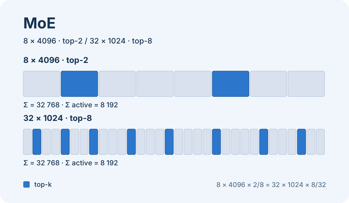
Consider this illustrative comparison between two layer designs:

Experts available — Larger experts: 8; Four-times-finer granularity: 32

Experts selected per token — Larger experts: 2; Four-times-finer granularity: 8

Intermediate width of each expert — Larger experts: 4,096; Four-times-finer granularity: 1,024

Sum of available widths — Larger experts: 32,768; Four-times-finer granularity: 32,768

Sum of selected widths — Larger experts: 8,192; Four-times-finer granularity: 8,192

Possible sets of selected experts — Larger experts: 28; Four-times-finer granularity: 10,518,300

The numbers were chosen to explain the transformation; they do not describe a model measured here. The last calculation is combinatorial: choosing 2 out of 8 or 8 out of 32, without counting order or combination weights.

For FFNs in the same family and with the same input dimension, these sums help compare expert parameters and multiplications, ignoring biases and other terms. They do not count the router, dispatch, communication, or kernel efficiency.

The second design can choose more varied combinations of smaller transformations. This creates potential flexibility; it does not turn millions of combinations into millions of demonstrated skills. Training must learn to use them.

Shared experts and balancing

Shared experts run for all tokens in the layers that include them. Routed experts are selected dynamically. The proposal seeks to reduce repetition of common functions among experts and leave more room for differentiation. DeepSeek-V2 combines this FFN organization with MLA in attention. DeepSeek-V2 [35].

In the DeepSeekMoE budget comparison, reserving shared experts requires subtracting them from the active routed count. Otherwise, computation is added instead of merely reorganized. DeepSeekMoE, section 3.2 [33].

The router also has to handle load. If many tokens reach the same device, that destination can become the bottleneck. Work imbalance and specialization collapse are related but not identical problems.

DeepSeek-V3, at the end of 2024, uses bias adjustments to balance routing without relying on a main auxiliary balancing loss; the report still includes a small per-sequence auxiliary loss. It also limits the nodes to which a token is sent. “Auxiliary-loss-free” does not mean that training has no auxiliary loss at all. DeepSeek-V3 [36].

There are other choices. In Expert Choice, from 2022, each expert selects a set of tokens, allowing a token to receive different numbers of experts. This differs from per-token top-k and from a hierarchical tree. Restricting destinations by device or node, in turn, does not prove the existence of a tree of semantic specializations. Expert Choice Routing [37].

Active parameters are not total memory

Activating fewer experts may reduce FFN computation per token. The weights of the other experts still exist: they have to reside somewhere and be available when selected.

Distributing them across devices introduces dispatch and communication, often with exchanges among many destinations. Keeping them outside fast memory may introduce transfers and latency. The final gain depends on batch size, interconnect, token distribution, and runtime. Communication engineering itself occupies an important part of scaling work. GShard [13].

An MoE with 37B active parameters cannot automatically be treated as a 37B dense model in memory or speed requirements.

2024–2026: the lines coexist within the same model

Jamba, presented in 2024, combines Mamba and Transformer layers, with MoE in part of the transformations. It clearly shows that “recurrent,” “attention,” and “experts” are not mutually exclusive categories. Attention layers still have their cache; recurrent layers have their own state. Jamba [38].

Compressing KV and selecting context: MLA, NSA, and DSA

DeepSeek-V2's MLA, in 2024, compresses the per-position KV representation into a latent space, with its own treatment of positional information. It reduces the amount stored per token; it does not automatically make the number of retained positions constant. DeepSeek-V2 [35].

In 2025, Native Sparse Attention investigated combining compression, selection, and local access in a hardware-aligned design. DeepSeek Sparse Attention, described in the V3.2 report, uses an indexer to select positions that reach the main attention. Selecting fewer positions does not eliminate the cost of selecting them: the whole system must be examined before promising linear complexity or speed. NSA [39], DeepSeek-V3.2 [40].

Three current examples, with public configurations

Qwen3.5-35B-A3B-Base, 2026. The model card describes 40 layers organized in groups of three Gated DeltaNet layers for one Gated Attention layer, with MoE in both types. It reports 35B total parameters, approximately 3B active, and, in the MoE layers, eight active routed experts and one shared expert. It is a concrete combination of recurrent memory, attention, and FFN selection. Model card [41], official configuration [42].

MiMo-V2-Flash, January 2026 report. It combines MoE with 309B total parameters and 15B active parameters, with sliding-window attention and global attention. The report describes a ratio of five local layers to one global layer. This reduces local reach per layer without making every layer local attention. The proportions of one version should not automatically be copied to the whole MiMo family. Report [43].

DeepSeek-V4, released in April 2026. The vendor's card keeps DeepSeekMoE and describes hybrid attention with CSA and HCA. CSA compresses the sequence and applies sparse selection; HCA uses stronger compression with dense attention over the compressed representation. The card reports 1.6 trillion total parameters and 49B active for the Pro variant. Official technical card [44].

V4 also introduces mHC, which reorganizes communication among residual streams with constraints on their mixing. This acts on another architectural axis: the circulation of representations among blocks, beyond expert selection and context access. The implementation documentation makes these components explicit. DeepSeek-V4 in Transformers [45].

The attention paths of these models still store KV information. In the Qwen cited, recurrent-layer state and attention-layer KV behave differently. In MiMo, the window limits local blocks while global blocks have another reach. In V4, compression and selection reduce the volume consulted; they do not make all storage independent of history.

These examples are documented configurations, not a quality ranking. Active parameters, number of experts, and advertised context are not interchangeable benchmarks.

2024–2026: depth, processing unit, and generation also change

The map remains incomplete if we look only at FFNs and attention. Other lines change where computation is spent and how output is produced.

Depth recurrence: reusing transformations across multiple passes over a representation has precedents such as Universal Transformers, from 2018. In 2025, a study of recurrent depth explored increasing computation in latent space by repeating a block instead of relying only on producing more tokens. Reusing weights reduces the need for distinct parameters for every pass, but repeating the block still costs computation. It is another research axis, different from carrying state across tokens. Universal Transformers [46], recurrent depth, 2025 [47].

Mixture-of-Depths, 2024: selects which tokens participate in operations of particular layers under a budget. The selection changes the distribution of computation through depth; it is not simply choosing experts inside an FFN. MoD [48].

Byte Latent Transformer, 2024: groups bytes into variable-length patches and performs an important part of processing on those representations, with local components for input and output. Here the unit on which more expensive computation is organized also changes. BLT [49].

Multi-Token Prediction, 2024: adds objectives and modules to predict more than one future token. Training must be separated from the use of these modules during generation. Gloeckle and colleagues' work presents this investigation; in DeepSeek-V3, the modules can be discarded at inference or used to support speculative decoding. Therefore, saying that MTP “changes nothing in inference” is too absolute. MTP [50], use in V3 [36].

Diffusion for language, such as LLaDA, 2025: explores reconstructing masked tokens instead of only continuing from left to right. It may use a Transformer backbone, but changes the objective and generation process. Refining several positions in stages has different costs from generating one token per step; lower latency should not be assumed merely because parallelism is possible. LLaDA [51].

Memory learned during use, such as Titans, at the turn of 2024 to 2025: investigates long-term memory modules updated at test time. This type of memory is not an external document database and not merely the KV cache. It is a research line with its own update rules, cost, and evaluation. Titans [52].

In 2026, Mamba-3 also continues developing the state-space line. The existence of a new paper expands the map, but does not prove widespread adoption or superiority over models at different scales and tasks. Mamba-3 [53].

The timeline, without turning branches into replacements

1990–1997: recurrence and LSTM — What becomes possible to investigate or organize more clearly: Carrying and controlling state while processing sequences.

1991–1994: mixtures of experts — What becomes possible to investigate or organize more clearly: Dividing and combining learned functions, including hierarchically.

2014: seq2seq and attention — What becomes possible to investigate or organize more clearly: Transforming sequences and consulting input positions during generation.

2017: sparse-gated MoE and Transformer — What becomes possible to investigate or organize more clearly: Scaling subnetwork selection and reorganizing communication among positions.

2018–2019: GPT, BERT, and T5 — What becomes possible to investigate or organize more clearly: Exploring decoders, encoders, and encoder-decoder combinations.

2019–2023: MQA, sparse attention, FlashAttention, and GQA — What becomes possible to investigate or organize more clearly: Reducing KV, choosing connections, and improving execution through distinct mechanisms.

2020–2024: linear attention, S4, Mamba, and SSD — What becomes possible to investigate or organize more clearly: Updating structured memory and bringing recurrent and parallel perspectives closer.

2024: fine-grained MoE, MLA, Jamba, and DeltaNet — What becomes possible to investigate or organize more clearly: Refining experts, compressing KV, combining operators, and controlling memory writing.

2024–2025: MoD, BLT, MTP, and diffusion — What becomes possible to investigate or organize more clearly: Changing executed depth, processing unit, and generation.

2025–2026: NSA, DSA, LFM2, and recent public hybrids — What becomes possible to investigate or organize more clearly: Combining these choices in specific model configurations.

The years indicate the milestones discussed and their sources, not a claim that every idea began there. There are earlier works, later versions, and other lineages. The chronology explains how the mechanisms connect; it does not establish a winner.

How to read a model's architecture without getting lost in the names

Instead of asking only whether a model is dense or MoE, look for answers to five questions:

1. How do positions exchange information? Full attention, windows, sparse selection, convolution, recurrence, or a combination? 2. Which transformations are executed? Dense FFNs, routed experts, shared experts, or variable depth? 3. What grows with history? KV per position, compressed representations, recurrent state, and local buffers need to be separated. 4. How does the model learn and generate? Next token, MTP, diffusion, and speculative decoding are not the same decision. 5. Which implementation supported the results? Numerical precision, batch, context, kernels, and hardware define the observed cost.

To compare efficiency, measure prefill, per-token latency, throughput, memory, and quality on relevant tasks under equivalent conditions. A laboratory result or an active-parameter number does not by itself demonstrate a general improvement.

The most interesting advance in this path is the freedom to compose: use smaller experts where their combination helps, recurrent memory where state is enough, and more direct context access where it is needed. Each choice must justify what it preserves, what it compresses, and what it costs when the model actually starts working.